
NOTE: The python example code for this technical
blog can be found in this GitHub repo:
Consider the following situation; you have some data loaded into Apache Beam which you need to process. You have some value in the source data which you want to use to find a unique row in a BigQuery table. Consider the following source data.
| Row UUID | Country | Year | Cheese consumption per capita per year (kg) |
| 1 | The Netherlands | 2011 | 19.4 |
| 2 | The Netherlands | 2012 | 20.1 |
| 3 | France | 2011 | 26.3 |
| 4 | China | 2011 | 0.1 |
Table 1. Source data
The Challenge
We want to look up in which continent the countries described in the table above reside for each row. As an example we have the following table from some data source (e.g. BigQuery, json etc.):
| Country | Continent |
| The Netherlands | Europe |
| China | Asia |
| France | Europe |
| Brazil | South America |
Table 2. Join Data
We need to left join on country to find the correct continent. In SQL, a left join is a command to join two tables with a common column. The SQL command would be:
SELECT Row UUID, Country, Year, Cheese consumption per capita per year (kg)
FROM table1
LEFT JOIN table2 ON table1.Country = table2.Country;
We want to join the first table with the second table on the Country column. This would result in following joined table:
| Row UUID | Country | Year | Cheese consumption per capita per year (kg) | Continent |
| 1 | The Netherlands | 2011 | 19.4 | Europe |
| 2 | The Netherlands | 2012 | 20.1 | Europe |
| 3 | France | 2011 | 26.3 | Europe |
| 4 | China | 2011 | 0.1 | Asia |
The left join is a build-in function in SQL and is very useful to match records from 1 table with another in relational databases. In Apache Beam however there is no left join implemented natively. There is however a CoGroupByKey PTransform that can merge two data sources together by a common key.
How to implement a left join using the python version of Apache Beam
The overall workflow of the left join is presented in the dataflow diagram presented in Figure 1.

Figure 1. Overall Dataflow Diagram
(Click to enlarge)
In a production environment you would typically have data in some file format (e.g. csv, json, txt) which you have read using for example the build-in ReadFromText module of Apache Beam IO and do some processing using DoFn’s to format it as a pcollection of dictionaries.
CoGroupByKey explained
In order to use the CoGroupByKey PTransform, we need to format the read data as common (key, value) tuples. The read data from 2 or more sources are grouped together by the common key. Figure 2 shows what the CoGroupByKey looks like in python syntax, where we have 2 element tuples to be cogrouped. Each 2-element tuple must contain a key to be grouped. The first element of the tuple is the key and the second element of the tuple is the object you want to group. It can be any serializable object. The grouped tuple contains (for every unique key) one 2-element tuple where the second element is a dictionary where the keys are the names of the data sources and the values are a list of all the second elements of the set of all data source tuples you want to cogroup.
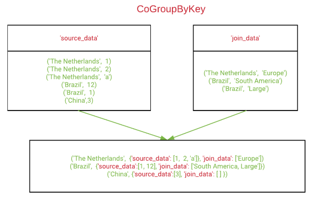 Figure 2. CogroupByKey Diagram
Apache Beam’s built-in CoGroupByKey core Beam transform forms the basis of a left join. The objects we want to cogroup are in case of a LeftJoin dictionaries. Example source data tuples:
('The Netherlands', {'Country': 'The Netherlands', 'Year': '2011','Cheese consumption
per capita per year (kg)': '19.4'})
('The Netherlands', {'Country': 'The Netherlands', 'Year': '2012','Cheese consumption
per capita per year (kg)': '20.1'})
Example join data tuple:
('The Netherlands', {'Country': 'The Netherlands', 'Continent': 'Europe'})
Example grouped tuple:
('The Netherlands', {'source_data': [{'Country': 'The Netherlands', 'Cheese consumption
per capita per year (kg)': '20.1', 'Year': '2012'}, {'Country': 'The Netherlands',
'Cheese consumption per capita per year (kg)': '19.4', 'Year': '2011'}], 'join_data':
[{'Country': 'The Netherlands', 'Continent': 'Europe'}]})
We still need to unnest the CoGroupBykey output to get the original source data. So our grouped tuple has to become like the following:
{'Country': 'The Netherlands', 'Cheese consumption per capita per year (kg)':
'19.4', 'Continent': 'Europe', 'Year': '2011'}
{'Country': 'The Netherlands', 'Cheese consumption per capita per year (kg)':
'20.1', 'Continent': 'Europe', 'Year': '2012'}
We will explain how to implement the entire left join process in Apache Beam.
How to implement Left Join using CoGroupByKey
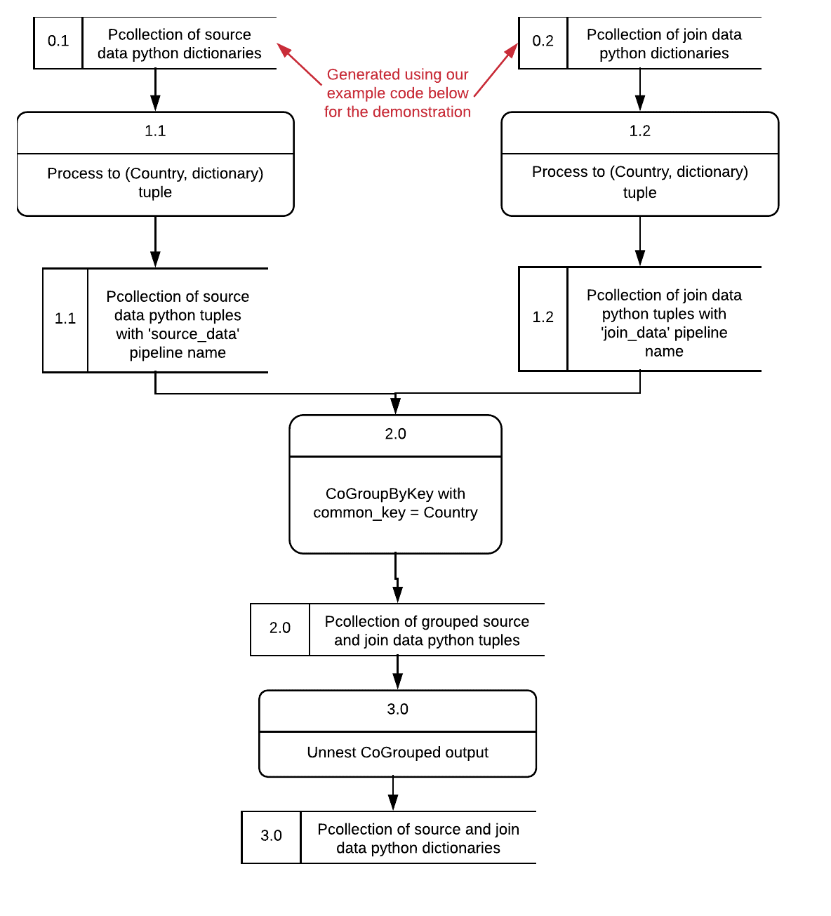
Figure 3. Overall Join Dataflow Diagram
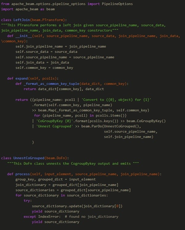
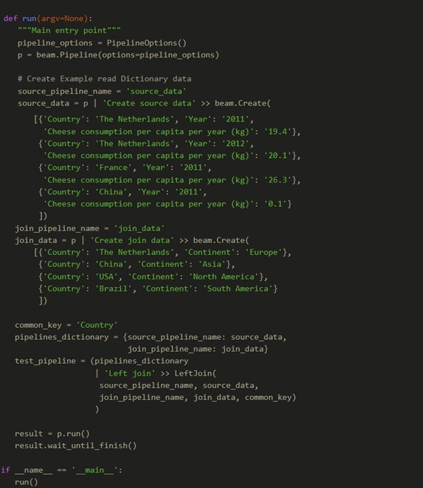
The Dataflow diagram of the join process is presented in Figure 3. The join process has 4 processing steps consisting of steps 1.1, 1.2, 2.0 and 3.0. Steps 1.1 and 1.2 run in parallel and steps 2.0 and 3.0 run after each other. We are now going to walkthrough the transformation process of the dataflow diagram in Figure 3. At step 0.1 and 0.2 we have (for illustration purposes) the source_data and join_data pcollection. For the purpose of our example implementation we generate these read elements ourselves. The following code creates the example dictionaries in Apache Beam, puts them into a pipelines_dictionary containing the source data and join data pipeline names and their respective pcollections and performs a Left Join.
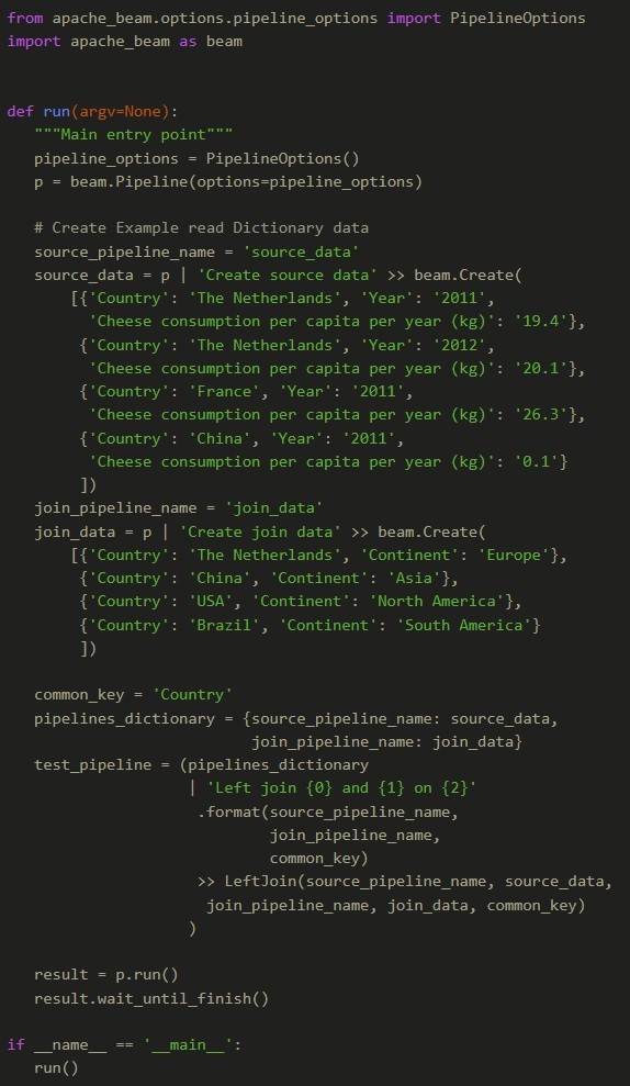
The code above can be found as part of the example code on the GitHub repo
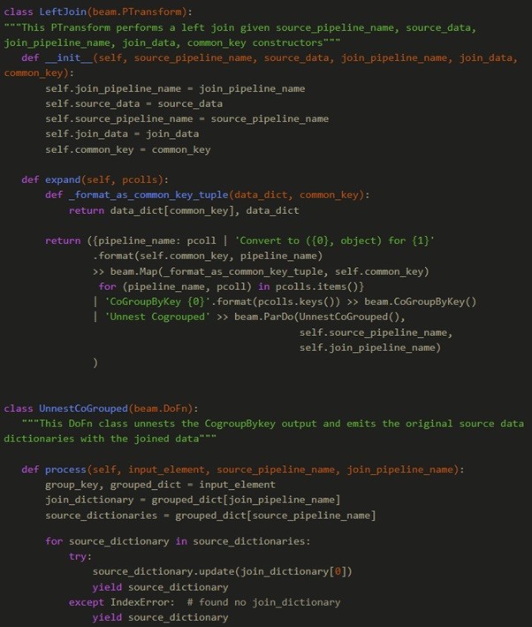
The LeftJoin is implemented as a composite PTransform. The composite PTransform takes as input a pipelines_dictionary containing the source_pipeline_name, source_data pcollection, join_pipeline_name and join_data pcollection.

The code above can be found as part of the example code on the GitHub repo
It also needs source_pipeline_name, source_data, join_pipeline_name, join_data and common_key as constructor variables. An example walkthrough of the transformations that happen with the data is as follows.
For example:
{'Country': 'The Netherlands', 'Year': '2011',
 'Cheese consumption per capita per year (kg)': '19.4'}
{'Country': 'The Netherlands', 'Year': '2012',
'Cheese consumption per capita per year (kg)': '20.1'}
{'Country': 'France', 'Year': '2011',
'Cheese consumption per capita per year (kg)': '26.3'}
{'Country': 'China', 'Year': '2012',
'Cheese consumption per capita per year (kg)': '0.1'}
and
{'Country': 'The Netherlands', 'Continent': 'Europe'}
{'Country': 'China', 'Continent': 'Asia'}
{'Country': 'USA', 'Continent': 'North America'}
{'Country': 'Brazil', 'Continent': 'South America'}
becomes
('Brazil', {'source_data': [], 'join_data': [{'Country': 'Brazil',
'Continent': 'South America'}]})
('USA', {'source_data': [], 'join_data': [{'Country': 'USA',
'Continent': 'North America'}]})
('The Netherlands', {'source_data': [{'Country': 'The Netherlands',
'Cheese consumption per capita per year (kg)': '20.1', 'Year': '2012'},
{'Country': 'The Netherlands', 'Cheese consumption per capita
per year (kg)': '19.4', 'Year': '2011'}], 'join_data': [{'Country':
'The Netherlands', 'Continent': 'Europe'}]})
('China', {'source_data': [{'Country': 'China',
'Cheese consumption per capita per year (kg)': '0.1',
'Year': '2011'}], 'join_data': [{'Country': 'China',
'Continent': 'Asia'}]})
('France', {'source_data': [{'Country': 'France',
'Cheese consumption per capita per year (kg)': '26.3',
'Year': '2011'}], 'join_data': []})
From here onwards we unnests the source data dictionaries and update them with the matched joined data dictionary. We then emit the updated source data dictionaries. The output will then be:
{'Country': 'The Netherlands', 'Year': '2011',
'Cheese consumption per capita per year (kg)': '19.4', 'Continent': 'Europe'}
{'Country': 'The Netherlands', 'Year': '2012',
'Cheese consumption per capita per year (kg)': '20.1', 'Continent': 'Europe'}
{'Country': 'France', 'Year': '2011',
'Cheese consumption per capita per year (kg)': '26.3'}
{'Country': 'China', 'Year': '2011',
'Cheese consumption per capita per year (kg)': '0.1', 'Continent': 'Asia'}
The PTransform code uses 2 classes, namely the LeftJoin Ptransform class and the UnnestCoGrouped DoFn class. The LeftJoin is a Composite PTransform that uses dictionary comprehension and Map to format the source and join data as suitable cogroupby tuples. It then uses the built-in CoGroupByKey PTransform to group them together by common_key. The last part is to unnest the grouped dictionaries and emit the updated dictionaries which is done using the UnnestCogrouped DoFn.
The code above can be found as part of the example code on the GitHub repo
The full example code block to run this example is given below:
The code above can be found as part of the example code on the GitHub repo
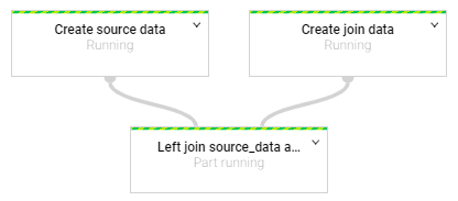
If you run this example you would have the following Graph in Dataflow:
Which can be magnified by clicking on the down arrow next to the Left Join node:
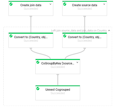
Exposing the nested logic of the implemented Leftjoin PTransform.
If you want to use the implemented LeftJoin, you would need the LeftJoin PTransform class and the UnnestCoGrouped DoFn class. Use the full code as an example guide to use the LeftJoin PTransform. This completes the walkthrough of implementing a LeftJoin in the python version of Apache Beam.
Conclusion
In short, this article explained how to implement a leftjoin in the python version of Apache Beam. The user can use the provided example code as a guide to implement leftjoin in their own Apache Beam workflows. If you want to learn more about Apache Beam, click here to get all the Apache Beam resources.
Related Google Cloud Technical blog-posts
- Creating a master orchestrator to handle complex Google Cloud Composer jobs
- Creating complex orchestrations with Google Cloud Composer using sub_controllers
- Google Cloud: Infrastructure as Code with Terraform
- Creating anonymized Primary keys for Google BigQuery
Join our open & innovative culture
Open, accessible and ambitious are the keywords of our organizational culture. We encourage making mistakes, we strive to do better every day and love to have fun. Doing work you love with brilliant people is what it’s all about.

